Example configurations

Next, we will investigate a number of pre-configured example files that are shipped with Kassiopeia. These files serve as a working example of various features of the simulation, but also as a reference for your own configurations. Please take some time to investigate these example files.

The example configurations can be found online at GitHub: Kassiopeia/XML/Examples and are installed to:

$KASPERSYS/config/Kassiopeia/Examples/

The Dipole Trap Example 

The first example is a simulation of a simple dipole trap, or rather, a magnetic mirror device. It consists of two dipole magnets positioned some distance apart along the same axis to form a magnetic bottle. To make the simulation slightly less trivial and more suitable to show Kassiopeia features, a ring electrode has been added near the center of the magnetic bottle emulating a MAC-E filter spectrometer. To run this simulation type:

Kassiopeia $KASPERSYS/config/Kassiopeia/Examples/DipoleTrapSimulation.xml

On the first run of this simulation, Kassiopeia will call KEMField to solve the static electric and magnetic fields of the geometry and compute zonal harmonic (an axially symmetric approximation) coefficients. Once field solving is finished, particle tracking of 1 event will commence.

Ignoring the messages from KEMField, the terminal output of this example will look something like:

[KSMAIN NORMAL MESSAGE] ☻  welcome to Kassiopeia 3.7  ☻
****[KSRUN NORMAL MESSAGE] processing run 0...
********[KSEVENT NORMAL MESSAGE] processing event 0 <generator_uniform>...
************[KSTRACK NORMAL MESSAGE] processing track 0 <generator_uniform>...
[KSNAVIGATOR NORMAL MESSAGE]   child surface <surface_downstream_target> was crossed.
************[KSTRACK NORMAL MESSAGE] ...completed track 0 <term_downstream_target> after 48714 steps at <-0.000937309 -0.000478289 0.48>
********[KSEVENT NORMAL MESSAGE] ...completed event 0 <generator_uniform>
****[KSRUN NORMAL MESSAGE] ...run 0 complete
[KSMAIN NORMAL MESSAGE] finished!
[KSMAIN NORMAL MESSAGE] ...finished

Once particle tracking has terminated you will find a .root output file located at:

$KASPERSYS/output/Kassiopeia/DipoleTrapSimulation.root

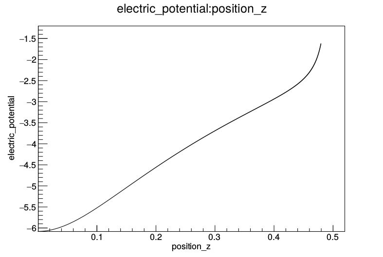
This file contains the data pertaining to the particle’s state during tracking, saved in the ROOT TTree format. The contents of the output file are configured in the XML file. The ROOT file maybe opened for quick visualization and histogramming using the ROOT TBrowser or other suitable tool, or it may be processed by an external analysis program. As an example, plotting the electric potential experienced by the electron as a function of its $z$ position produces the following graph.

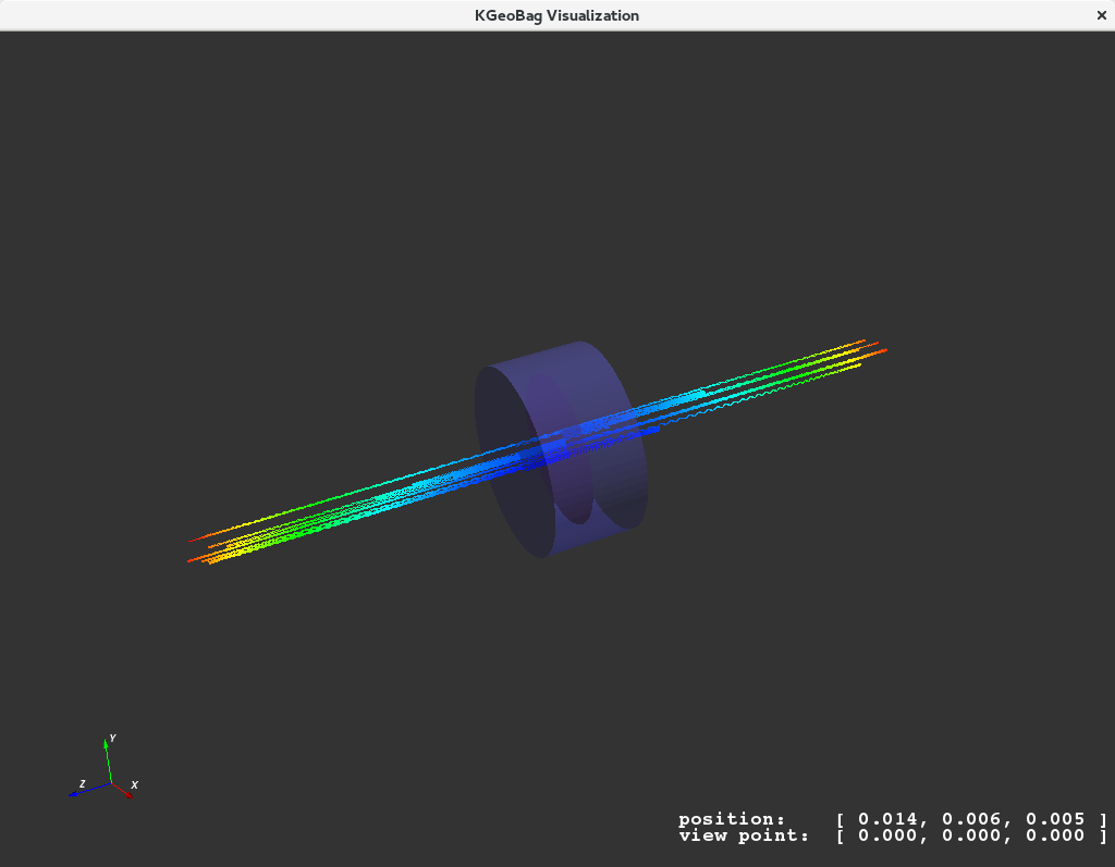
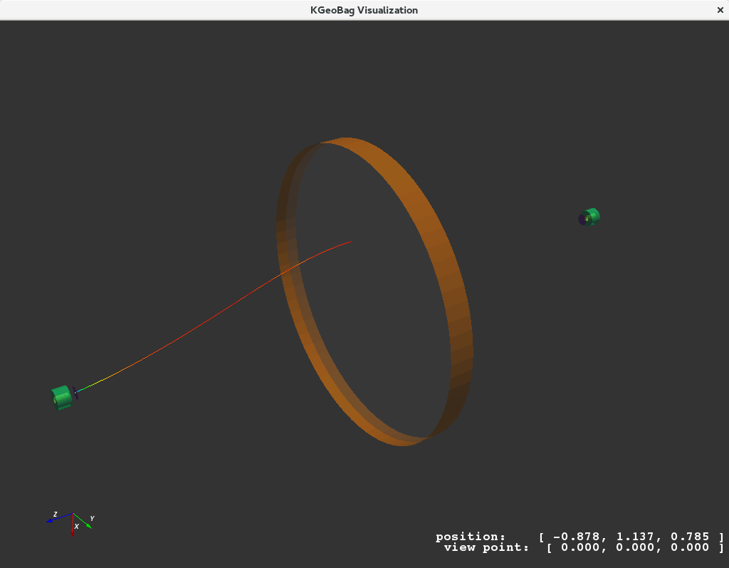
Trajectory Visualization 

For more advanced visualization Kassiopeia may be linked against the VTK library. If this is done, the DipoleTrapSimulation.xml example will include a configuration which will open an interactive VTK visualization window upon completion of the simulation. The output of which shows the electron’s track colored by angle between its momentum vector and the magnetic field. The following image demonstrates the VTK visualization of the simulation.

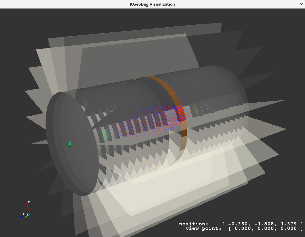
The Quadrupole Trap Example 

The second example to demonstrate the capabilities of Kassiopeia is that of a quadrupole (Penning) trap. This sort of trap is similar to those which are used to measure the electron $g$-factor to extreme precision. To run this example, locate the XML file in the config directory, and at the command prompt enter:

Kassiopeia $KASPERSYS/config/Kassiopeia/Examples/QuadrupoleTrapSimulation.xml

This example also demonstrates the incorporation of discrete interactions, such as scattering off residual gas. If VTK is used, upon the completion of the simulation a visualization window will appear. An example of this shown in the following figure. The large green tube is the solenoid magnet, while the amber hyperboloid surfaces within it are the electrode surfaces. The electron tracks can be seen as short lines at the center.

Simulation Analysis 

Furthermore, a very simple analysis program example QuadrupoleTrapAnalysis can be run on the resulting .root file. To do this, execute the following after the output file was created:

QuadrupoleTrapAnalysis $KASPERSYS/output/Kassiopeia/QuadrupoleTrapSimulation.root

The output of which should be something to the effect of:

extrema for track <1.43523>

This program can be used as a basis for more advanced analysis programs, as it demonstrates the methods needed to iterate over the particle tracking data stored in a ROOT TTree file. It is also possible to access the ROOT TTree data by other means, e.g. using Python scripts and the PyROOT or uproot modules, but this is out of scope for this section.

Analysis can also be performed by other means, e.g. in a Python notebook. An example for the quadrupole trap simulation is available in: QuadrupoleTrapAnalysis.ipynb

The Photomultiplier Tube Example 

As a demonstration of some of the more advanced features of Kassiopeia (particularly its 3D capabilities), an example of particle tracking in a photomultiplier tube is also included. This convifuration was also featured in the Kassiopeia paper [*].

Since the dimensions of the linear system that needs to be solved in order to compute the electric field is rather large (~150K mesh elements), the initialization of the electric field may take some time. If the user has the appropriate device (e.g. a GPU) it is recommended that the field solving sub-module KEMField is augmented with OpenCL in order to take advantage of hardware acceleration. This is done by setting the KEMField_USE_OpenCL flag in the build stage.

To run this simulation, type:

Kassiopeia $KASPERSYS/config/Kassiopeia/Examples/PhotoMultiplierTubeSimulation.xml

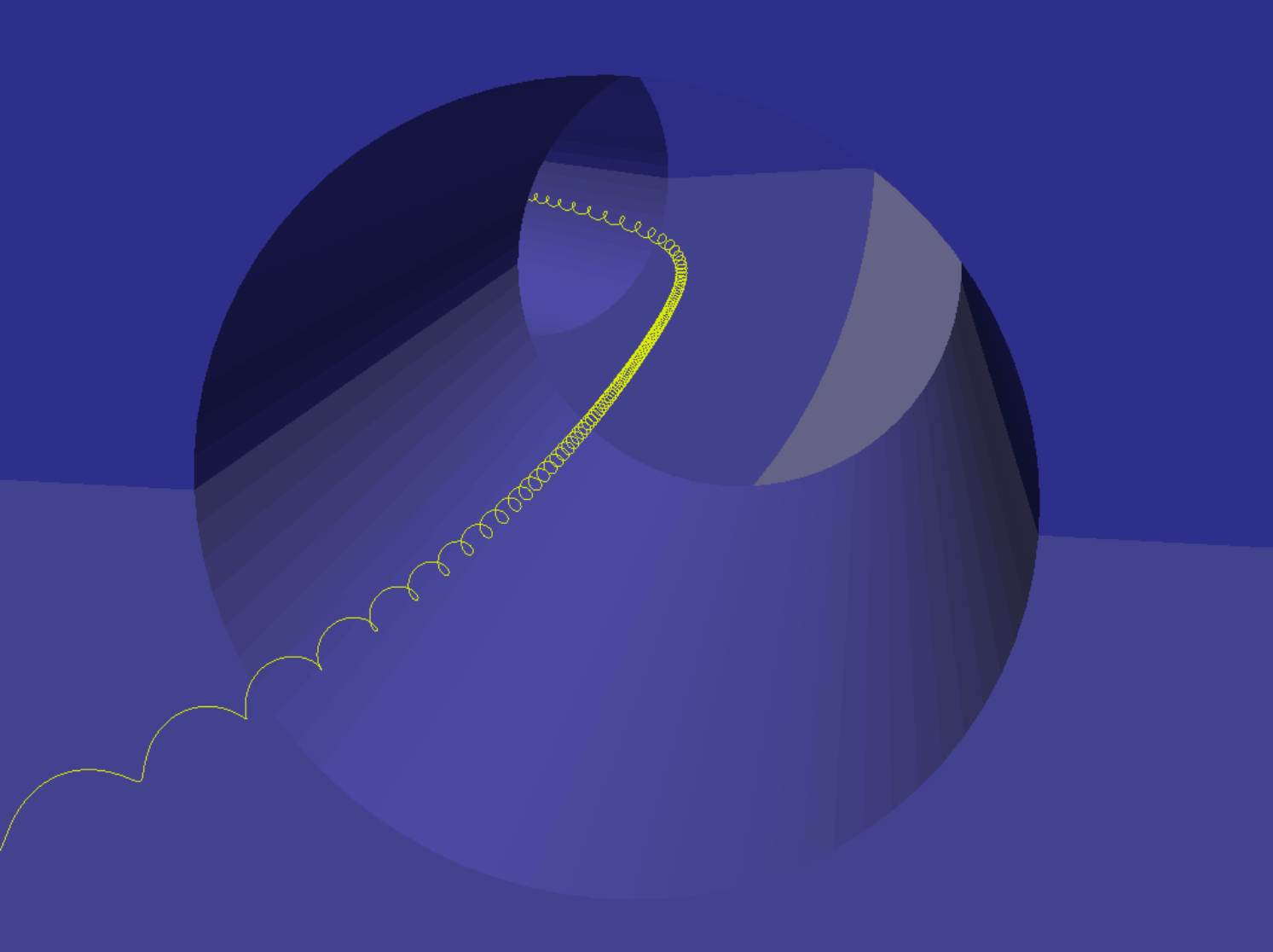
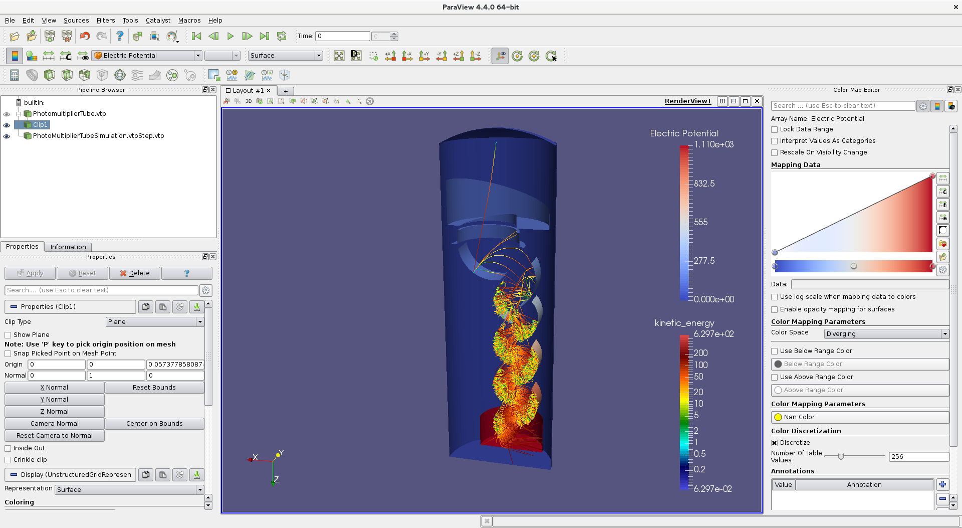
Visualization with ParaView 

Depending on the capability of your computer this example may take several hours to run, and you may want to execute it overnight. If you have enabled VTK, an .vtp output file called:

$KASPERSYS/output/Kassiopeia/PhotoMultiplierTubeSimulation.vtpStep.vtp

will be created. This file stores the particle step data for visualization using the VTK polydata format. Additionally, a file called PhotomultiplierTube.vtp will be created in the directory from which Kassiopeia was called. This file stores visualization data about the electrode mesh elements used by KEMField. Both of these files can be opened in the external program Paraview for data selection and viewing, or other suitable software. An example is shown in the following figure.

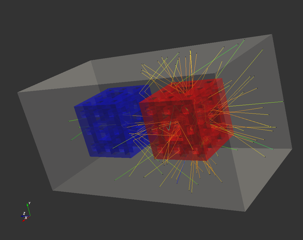
The Mesh Simulation Example 

The mesh simulation uses a geometry from an external STL file, which is a format widely used in 3D design software. The external geometry must provide a surface mesh in order to be usable with KEMField and Kassiopeia. In this example, an electric field is defined by two copies of the so-called Menger sponge cubes that are placed next to each other. Particles are tracked along a linear trajectory, which are reflected when they hit one of the cube surfaces.

Other Examples 

Some other examples which explore other concepts also distributed with Kassiopeia, and are described in the following table.

Other simulation examples
File	Description
`AnalyticSimulation.xml`	Quadrupole ion/electron trap (similar to the original `QuadrupoleTrapSimulation.xml`. However, the magnetic field is completely uniform and the and the electric field is described analytically as an ideal quadrupole.
`ToricTrapSimulation.xml`	This is a simulation of an electron trapped in a magnetic torus (similar to a Tokamak reactor), and it demonstrates the identification of surface intersections, as well as particle drift in non-homogeneous fields.
`DipoleTrapMeshedSpaceSimulation.xml`	This simulation has the same fields as the original ``DipoleTrapSimulation.xml`. However, there are additional (meshed, but non-interacting) surfaces present to demonstrate navigation in a complicated geometry using the meshed-surface octree-based navigator.