Understanding Simulation Output
This section provides a description of the output files created by a Kassiopeia simulation, along with examples to read and analyze the files.
Output configuration
Generally, Kassiopeia output is written to ROOT output (.root) files that store simulation data at the run, event, track and step level. In addition, if Kassiopeia was compiled with VTK support, output files in VTK polydata (.vtp) format may be written. These files are mainly intended for visualization, e.g. with the ParaView software. It is also possible to write simulation data as plaintext ASCII files, however this is not recommened for large simulations.
As explained in Configuring Your Own Simulation, the output format is configured by the available writers. Writers use the description of the output format in the XML configuration file, which specifies the output fields that will be written to file. Different output descriptions may be used for different writers.
Groups and fields
Structured output formats like ROOT and VTK allow to combine several output fields into a common group. This is not only useful for analyzing the simulation results, but also allows to distinguish between data produces at the run, event, track and step levels. An output group may be defined by the structure:
<output_group name="output_step_world">
    <output name="step_id" field="step_id" parent="step"/>
</output_group>
or, alternatively in the older XML syntax:
<ks_component_group name="output_step_world">
    <output name="step_id" field="step_id" parent="step"/>
</ks_component_group>
In this case, the output file will have one group output_step_world that contains one member field step_id and is updated at the step level, meaning that one entry will be added to the member field with each simulation step.
In the case above, the member field step_id refers to an attribute of the step class KSStep. Similar fields are available in the other classes, such as KSTrack. However, in a typical simulation one also wants to access physical attributes of the simulated particle. This is possible at the step level as well. In this case, one may access the initial or final state of the particle in each step (where the initial state of one step equals the final state of the preceding step, unless it is the first step in which the particle was generated). For example:
<output name="step_initial_particle" field="final_particle" parent="step"/>
<output name="step_final_particle" field="final_particle" parent="step"/>

<output_group name="output_step_world">
    <output name="step_id" field="step_id" parent="step"/>
    <output name="initial_position" field="position" parent="step_initial_particle"/>
    <output name="final_position" field="position" parent="step_final_particle"/>
</output_group>
writes the initial and final particle position at each step to file. Note that in this case, one must declare a member field step_…_particle that can be referenced inside the output group. Because the declaration is outside the group it is not written to file, and so the output file will contain three fields at the step level. The at the track level:
<output name="track_initial_particle" field="initial_particle" parent="track"/>
<output name="track_final_particle" field="final_particle" parent="track"/>

<output_group name="output_track_world">
    <output name="track_id" field="track_id" parent="track"/>
    <output name="initial_position" field="position" parent="track_initial_particle"/>
    <output name="final_position" field="position" parent="track_final_particle"/>
</output_group>
Vector data like the particle position is stored as an array of (x,y,z) components for each entry. Similarly, tensor data is stored as an array of nine components. One may also store derived attributes like magnitude or radius:
<output name="step_initial_particle" field="final_particle" parent="step"/>
<output name="initial_position" field="position" parent="step_initial_particle"/>

<output_group name="output_step_world">
    <output name="initial_position" field="position" parent="step_initial_particle"/>
    <output name="initial_radius" field="perp" parent="initial_position"/>
</output_group>
In addition to simple fields that reference internal attributes, some advanced calculation features are available:
math allows to evaluate arbitrary functions (using ROOT’s
TFormulaclass) that references one or more existing members.integral calculates the discrete integral of the referenced member field.
delta calculates the difference between the current value of a member field to the previous one.
minimum and maximum calculate the minimum/maximum value of a member field over the given interval (e.g. a track).
minimum_at and maximum_at calculate the position of the minimum/maximum value.
The example below shows usage of these advanced fields:
<output name="step_final_particle" field="final_particle" parent="step"/>
<output name="step_kinetic_energy" field="kinetic_energy_ev" parent="step_final_particle"/>
<output name="step_polar_angle_to_b" field="polar_angle_to_b" parent="step_final_particle"/>

<output_group name="output_step_world">
    <output name="kinetic_energy" field="kinetic_energy_ev" parent="step_final_particle"/>

    <!-- change in kinetic energy at each step -->
    <output_delta name="kinetic_energy_change" parent="step_kinetic_energy"/>

    <!-- longitudinal kinetic energy at each step, derived from kinetic energy and pitch angle -->
    <output_math name="long_kinetic_energy" term="x0*cos(x1*TMath::Pi()/180.)*cos(x1*TMath::Pi()/180.)"
            parent="step_kinetic_energy" parent="step_polar_angle_to_b"/>
</output_group>

<output name="step_length" field="continuous_length" parent="step"/>

<output_group name="output_track_world">
    <!-- value and position of minimum/maximum kinetic energy over each track -->
    <output_maximum name="max_kinetic_energy" group="output_step_world" parent="kinetic_energy"/>
    <output_minimum name="min_kinetic_energy" group="output_step_world" parent="kinetic_energy"/>
    <output_maximum_at name="max_kinetic_energy_position" group="output_step_world" parent="kinetic_energy"/>
    <output_minimum_at name="min_kinetic_energy_position" group="output_step_world" parent="kinetic_energy"/>

    <!-- integrated length of all steps in each track -->
    <output_integral name="total_length" parent="step_length"/>
</output_group>
Output structure
For the remainder of this section, we will refer to the QuadrupoleTrapSimulation.xml example file to discuss the
output fields and their structure. Here is the (slightly shortened) output confuguration of this example:
<output_group name="component_step_world">
    <output name="step_id" field="step_id" parent="step"/>
    <output name="continuous_time" field="continuous_time" parent="step"/>
    <output name="continuous_length" field="continuous_length" parent="step"/>
    <output name="number_of_turns" field="number_of_turns" parent="step"/>
    <output name="time" field="time" parent="component_step_final_particle"/>
    <output name="position" field="position" parent="component_step_final_particle"/>
    <output name="momentum" field="momentum" parent="component_step_final_particle"/>
    <output name="magnetic_field" field="magnetic_field" parent="component_step_final_particle"/>
    <output name="electric_field" field="electric_field" parent="component_step_final_particle"/>
    <output name="electric_potential" field="electric_potential" parent="component_step_final_particle"/>
    <output name="kinetic_energy" field="kinetic_energy_ev" parent="component_step_final_particle"/>
</output_group>

<output_group name="component_step_cell">
    <output name="polar_angle_to_z" field="polar_angle_to_z" parent="component_step_final_particle"/>
    <output name="polar_angle_to_b" field="polar_angle_to_b" parent="component_step_final_particle"/>
    <output name="guiding_center_position" field="guiding_center_position" parent="component_step_final_particle"/>
    <output name="orbital_magnetic_moment" field="orbital_magnetic_moment" parent="component_step_final_particle"/>
</output_group>

<output name="z_length" field="continuous_length" parent="step"/>
<output_group name="component_track_world">
    <output name="creator_name" field="creator_name" parent="track"/>
    <output name="terminator_name" field="terminator_name" parent="track"/>
    <output name="total_steps" field="total_steps" parent="track"/>
    <output name="number_of_turns" field="number_of_turns" parent="track"/>
    <output name="initial_time" field="time" parent="component_track_initial_particle"/>
    <output name="initial_position" field="position" parent="component_track_initial_particle"/>
    <output name="initial_momentum" field="momentum" parent="component_track_initial_particle"/>
    <output name="initial_magnetic_field" field="magnetic_field" parent="component_track_initial_particle"/>
    <output name="initial_electric_field" field="electric_field" parent="component_track_initial_particle"/>
    <!-- ... skipped lines ... -->
    <output name="final_time" field="time" parent="component_track_final_particle"/>
    <output name="final_position" field="position" parent="component_track_final_particle"/>
    <output name="final_momentum" field="momentum" parent="component_track_final_particle"/>
    <output name="final_magnetic_field" field="magnetic_field" parent="component_track_final_particle"/>
    <output name="final_electric_field" field="electric_field" parent="component_track_final_particle"/>
    <!-- ... skipped lines ... -->
    <output name="z_length_internal" field="continuous_length" parent="track"/>
    <output_integral name="z_length_integral" parent="z_length"/>
</output_group>
The output structure (with some fields skipped) is as follows:
digraph output { node [fontname="helvetica", fontsize=10]; graph [rankdir="LR"] { rank=same "component_step_world" [shape="folder", style=filled, fillcolor=yellow]; "component_step_cell" [shape="folder", style=filled, fillcolor=yellow]; "component_track_world" [shape="folder", style=filled, fillcolor=yellow]; } { rank=same "step" [shape="rectangle", style=filled, fillcolor=lightskyblue]; "track" [shape="rectangle", style=filled, fillcolor=lightgreen]; "component_step_final_particle" [shape="note", style=filled, fillcolor=whitesmoke]; "component_step_position" [shape="note", style=filled, fillcolor=whitesmoke]; "component_step_length" [shape="note", style=filled, fillcolor=whitesmoke]; "component_track_initial_particle" [shape="note", style=filled, fillcolor=whitesmoke]; "component_track_final_particle" [shape="note", style=filled, fillcolor=whitesmoke]; "component_track_position" [shape="note", style=filled, fillcolor=whitesmoke]; "component_track_length" [shape="note", style=filled, fillcolor=whitesmoke]; "z_length" [shape="note", style=filled, fillcolor=whitesmoke]; } "component_step_world" -> "step_id" -> "step"; "component_step_world" -> "continuous_time" -> "step"; "component_step_world" -> "continuous_length" -> "step"; "component_step_world" -> "number_of_turns" -> "step"; "component_step_world" -> "time" -> "component_step_final_particle"; "component_step_world" -> "position" -> "component_step_final_particle"; "component_step_world" -> "momentum" -> "component_step_final_particle"; "component_step_world" -> "magnetic_field" -> "component_step_final_particle"; "component_step_world" -> "electric_field" -> "component_step_final_particle"; "component_step_world" -> "electric_potential" -> "component_step_final_particle"; "component_step_world" -> "kinetic_energy" -> "component_step_final_particle"; "component_step_cell" -> "polar_angle_to_z" -> "component_step_final_particle"; "component_step_cell" -> "polar_angle_to_b" -> "component_step_final_particle"; "component_step_cell" -> "guiding_center_position" -> "component_step_final_particle"; "component_step_cell" -> "orbital_magnetic_moment" -> "component_step_final_particle"; "component_track_world" -> "creator_name" -> "track"; "component_track_world" -> "terminator_name" -> "track"; "component_track_world" -> "total_steps" -> "track"; "component_track_world" -> "number_of_turns" -> "track"; "component_track_world" -> "initial_time" -> "component_track_initial_particle"; "component_track_world" -> "initial_position" -> "component_track_initial_particle"; "component_track_world" -> "initial_momentum" -> "component_track_initial_particle"; "component_track_world" -> "initial_magnetic_field" -> "component_track_initial_particle"; "component_track_world" -> "initial_electric_field" -> "component_track_initial_particle"; "component_track_world" -> "final_time" -> "component_track_final_particle"; "component_track_world" -> "final_position" -> "component_track_final_particle"; "component_track_world" -> "final_momentum" -> "component_track_final_particle"; "component_track_world" -> "final_magnetic_field" -> "component_track_final_particle"; "component_track_world" -> "final_electric_field" -> "component_track_final_particle"; "component_track_world" -> "z_length_internal" -> "track"; "component_track_world" -> "z_length_integral" -> "z_length"; "component_step_position" -> "step" [style=dashed]; "component_step_length" -> "step" [style=dashed]; "component_step_final_particle" -> "step" [style=dashed]; "z_length" -> "step" [style=dashed]; "component_track_position" -> "track" [style=dashed]; "component_track_length" -> "track" [style=dashed]; "component_track_final_particle" -> "track" [style=dashed]; "component_track_initial_particle" -> "track" [style=dashed]; }where the relations between the output groups (left), member fields (middle), and parent objects (right) are indicated by connecting arrows and the different node shapes. The output groups and fields are what is visible in the output file. Member fields either refer to a particle state of a step/track, or to attributes at the step/track level directly. The field z_length is a special case, since an intermediate field is necessary to perform the integration at track level.
ROOT output files
The ROOT output format is the standard file format that Kassiopeia produces. It supports flexible configuration,
structured data fields, and efficient storage on disk. The data fields are placed in ROOT’s TTree and TLeaf
objects that are created for each output group and member field, respectively.
Data structure
In the output file, several tree structures are present that open into a list of leafs, corresponding to the simulation
data. Here is an example view in the ROOT TBrowser:
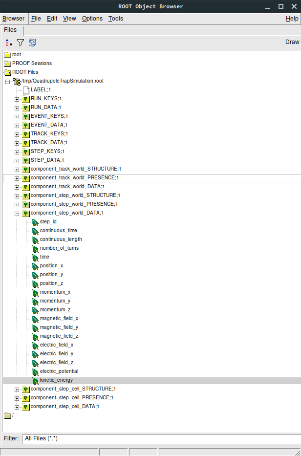
According to the configuration in QuadrupoleTrapSimulation.xml, three output groups have been created:
component_track_world, component_step_world, and component_step_cell. Each of these is split into several tree
in the ROOT file, distinguished by their postfix:
…_DATA contains the actual simulation data. For each output field, one leaf object (an array-like structure) is created in the output file. In the example shown here, the component_step_world_DATA tree contains the fields step_id, time and so on. In case of vector or tensor data, one individual field is created for each component, e.g. position_x, position_y, position_z. All output fields are sorted by the respective index, e.g. step data is sorted by STEP_INDEX (which is a continually increasing integer number). This allows direct access to any specific data field at any output level. Note that the step index can be different than the step id, which is an attribute of the KSStep class and thus defined by the simulation.
…_PRESENCE indicates which segments in the data array contain valid data. This tree contains the fields INDEX, referring to the start index in the output data, and LENGTH, referring to the length of one segment. When reading values from the data arrays, these fields should be checked so that only valid data is used.
…_STRUCTURE contains the fields LABEL and TYPE. For each output field present in the file, they indicate its name (i.e. the name of the leaf placed under …_DATA) and its type (
doubleetc.). When reading the data arrays, this information can be taken into account in order to treat data types correctly.
Note that the data in each leaf is written continuously, i.e. there is no distinction between individual tracks, events, or runs. This is done in order to improve storage efficiency and to provide a clean output structure. Hence, the step index is a monotonic integer number that increases with each new value written to the output file. In order to distinguish between different tracks, one needs to know the step indices corresponding to the start and end of the track so that the corresponding data segment can be analyzed. This is possible with the following meta-data fields.
In addition to the output groups defined in the XML configuration file, several trees containing meta-data are present in the output file. This data is always present in the ROOT file, regardless of the output configuration:
RUN_KEYS, EVENT_KEYS, etc. contain the names of the output groups present in the file. In the example shown here, the TRACK_KEYS tree contains one element component_track_world, while STEP_KEYS contains two elements.
RUN_DATA, EVENT_DATA, etc. each contain a list of run/event/… indices that correspond to the internally used indices for accessing data at the corresponding level. For example, STEP_DATA contains a field STEP_INDEX, which holds all indices that can be accessed in the data arrays. In addition, the …_DATA trees at higher levels than step also provide a mapping between to the indices at the lower levels:
TRACK_DATA contains the arrays FIRST_STEP_INDEX and LAST_STEP_INDEX. For each track that is designated by TRACK_INDEX they point to the index of the first and last step of the track. Hence if one looks at the step output, component_step_world in this case, one may use these step indices to split the step data into individual track segments. Similarly,
EVENT_DATA contains the fields (FIRST|LAST)_STEP_INDEX and (FIRST|LAST)_TRACK_INDEX, and
RUN_DATA contains (FIRST|LAST)_STEP_INDEX, (FIRST|LAST)_TRACK_INDEX, and (FIRST|LAST)_EVENT_INDEX.
Accessing simulation data
In most cases, for example when using the ROOT TBrowser, one may just look into the STEP_DATA and TRACK_DATA
fields to find the relevant information. For more sophisticated analyses, other means of accessing the data are
available.
Using Kassiopeia
Kassiopeia includes a simple analysis application that uses the KSReadFileROOT class to iterate through the step output produced by the QuadrupoleTrapSimulation.xml example. Its code is available at GitHub: Kassiopeia/Applications/Examples/Source/QuadrupoleTrapAnalysis.cxx and it serves as a general example of using this method.
In this case, the simulation output can be accessed in a structured way, using the run/event/track/step levels and iterating through each component:
for (tRunReader = 0; tRunReader <= tRunReader.GetLastRunIndex(); tRunReader++) {
    // run analysis code

    for (tEventReader = tRunReader.GetFirstEventIndex(); tEventReader <= tRunReader.GetLastEventIndex(); tEventReader++) {
        // event analysis code

        for (tTrackReader = tEventReader.GetFirstTrackIndex(); tTrackReader <= tEventReader.GetLastTrackIndex(); tTrackReader++) {
            // track analysis code

            for (tStepReader = tTrackReader.GetFirstStepIndex(); tStepReader <= tTrackReader.GetLastStepIndex();  tStepReader++) {
                // step analysis code
            }
        }
    }
}
Individual output fields are accessed via an instance of KSReadObjectROOT, as shown in the example. The benefit of using this method is that it uses Kassiopeia’s internal classes that are fully compatible with the writer class that produced the output file. On the other hand, it requires writing a custom C++ application that needs to be compiled against Kasper.
Using ROOT
Alternatively, the output can be access directly from a ROOT program. In this case, the ouput is accessible through the TTreeReader interface:
TFile file("QuadrupoleTrapSimulation.root");

TTreeReader track_data("TRACK_DATA", &file);
TTreeReaderValue<unsigned> first_step_index(track_data, "FIRST_STEP_INDEX");
TTreeReaderValue<unsigned> last_step_index(track_data, "LAST_STEP_INDEX");

TTreeReader step_data("component_step_cell_DATA", &file);
TTreeReaderValue<double> step_moment(step_data, "orbital_magnetic_moment");

TTreeReader step_presence("component_step_cell_PRESENCE", &file);
TTreeReaderValue<unsigned> valid_index(step_presence, "INDEX");
TTreeReaderValue<unsigned> valid_length(step_presence, "LENGTH");
As explained further below, here it is necessary to take into account the information from the TRACK_DATA tree to
get the first and last step index belonging to each track, as well as the ..._PRESENCE tree to only work on valid
entries in the output group. Because the simulation only fills the component_step_cell output in a certain region
of the geometry (the inner part of the trap), some values outside this region contain invalid values.
One approach to handle this structure is shown below, where the main loop iterates over each track and the inner loop over the steps only processes valid output fields:
vector<pair<unsigned,unsigned>> valid_steps;
while (step_presence.Next()) {
    valid_steps.emplace_back(*valid_index, *valid_index + *valid_length);
}

while (track_data.Next()) {
    auto max_moment = -TMath::Infinity();
    auto min_moment = TMath::Infinity();

    while (step_data.Next()) {
        auto index = step_data.GetCurrentEntry();

        if (index < *first_step_index)
            continue;
        if (index > *last_step_index)
            break;

        for (auto & valid : valid_steps) {
            if (index >= valid.first && index <= valid.second) {
                if (*step_moment > max_moment)
                    max_moment = *step_moment;
                if (*step_moment < min_moment)
                    min_moment = *step_moment;
            }
        }
    }
    auto deviation = 2.0 * (max_moment - min_moment) / (max_moment + min_moment);
    cout << "extrema for track <" << deviation << ">" << endl;
}
Using Python
Another common method of analysis makes use of Python libraries such as NumPy and Pandas. Several methods of getting the Kassiopeia output into a Python script are available:
KassiopeiaReader is a Python module based on PyROOT (the official Python-interface of the ROOT software). It is essentially a wrapper around ROOT classes that takes into account the relations between Kassiopeia’s output levels and allows easy iteration over step/track/… data fields. Its code is available at GitHub: Kassiopeia/Python/KassiopeiaReader.py.
uproot is a ROOT-less implementation of the ROOT file interface. It allows to access Kassiopeia’s output data without the ROOT dependency. Especially for large output files, this is a very efficient way of processing the simulation results. However, it is difficult to take into account relations between the output levels; e.g. in order to select specific steps that belong to a track or event in the simulation.
Pandas can be used together with uproot (or PyROOT) to access Kassiopeia’s output data in the form of a Pandas dataframe. With some extra work, it is possible to include the relations between output levels as well.
All three methods will be briefly explained in this section, in the form of a simple example that reproduces the
QuadrupoleTrapAnalysis.cxx code introduced above. The examples use the ROOT file QuadrupoleTrapSimulation.root
produced by the QuadrupoleTrapSimulation.xml example.
Using Python with KassiopeiaReader
The KassiopeiaReader Python module provides an iterator interface to a selected output group in a Kassiopeia
file. It can easily be used to retrieve e.g. all track or step output from a simulation. Correctly iterating over
more advanced output definitions take more effort, however. The QuadrupoleTrapSimulation is a good example for this,
because it uses an additional output region (component_step_cell) that is only filled with data in a small section
of each particle’s trajectory.
To re-implement the QuadrupoleTrapAnalysis.cxx program, a few things need to be considered that are explained below. The full example script is located at GitHub: Kassiopeia/Python/Examples/QuadrupoleTrapAnalysis.py.
import KassiopeiaReader

reader = KassiopeiaReader.Iterator('QuadrupoleTrapSimulation.root')

reader.loadTree('component_step_cell')
reader.select('orbital_magnetic_moment')

track_step_index = list(zip(*[reader.getTracks('FIRST_STEP_INDEX'), reader.getTracks('LAST_STEP_INDEX')]))

step_presence = reader.getTree('component_step_cell_PRESENCE')
step_valid = list(zip(*[step_presence['INDEX'], step_presence['LENGTH']]))
First of all, we need to import the Python module and create an instance for reading the output file
QuadrupoleTrapSimulation.root. The data we’re interested in is located in the component_step_cell tree.
As we will see later, the component_step_cell_PRESENCE tree is important in this example because it defines the
step entries that contain valid data (i.e. where the output was filled by the simulation, according to the definition
in the configuration file.) Because we’re only interested in a single output field orbital_magnetic_moment, we
can select it before accessing any data in order to reduce memory footprint.
Our analysis requires to compute the magnetic moment deviation for each single track. This requires to consider the
relation between step and track data. One method which is used here is to use the (FIRST|LAST)_STEP_INDEX field of
the track structure to select the first and last step index which belongs to a given track. However, because
not all of these steps will contain data in this case, some further adjustment is required: We also check the contents
of the component_step_cell_PRESENCE tree from above, and see if the first step index needs to be moved ahead to
the first valid data point. Similarly, we check if the last step index needs to be moved back.
for first_step_index, last_step_index in track_step_index:

    max_moment = -np.inf
    min_moment = np.inf

    for step in iter(reader):
        step_index = reader.iev - 1

        if step_index < first_step_index:
            continue

        for first_valid,valid_length in step_valid:

            last_valid = first_valid + valid_length - 1
            if step_index >= first_valid and step_index <= last_valid:

                moment = float(step.orbital_magnetic_moment)
                if moment > max_moment:
                    max_moment = moment
                if moment < min_moment:
                    min_moment = moment

            if first_valid > first_step_index:
                break

        if step_index >= last_step_index:
             break

    deviation = 2.0 * (max_moment - min_moment) / (max_moment + min_moment)
    print("extrema for track <{:g}>".format(deviation))
With this information, the step iterator can be advanced to the first step before starting the data processing. It is
then very straightforward to iterate over the range of steps beloging to the current track by advancing the step
iterator accordingly. In this example we retrieve the value orbital_magnetic_moment for each step, determine
its minimum/maximum over the entire track, and then calculate and print a mean deviation.
All output values should be in agreement with the C++ program.
Using Python with uproot / Pandas
The same result can be achieved by using the uproot package with Pandas dataframes. In this case, PyROOT isn’t needed and the analysis can run without ROOT dependencies. Applying the knowledge about Kassiopeia’s output structure that we gathered in the section above, we can write the following snippet:
import numpy as np
import uproot
#import uproot3 as uproot  # try this if newer uproot does not work

# Open data file
data = uproot.open('QuadrupoleTrapSimulation.root')

# Read data structures
df0 = data['TRACK_DATA'].pandas.df()
df1 = data['component_step_cell_DATA'].pandas.df()
df1p = data['component_step_cell_PRESENCE'].pandas.df()

# Extend step data for merging
df1.assign(track_id=np.nan)

# Iterate over tracks and assign to step data
for track_id, first_step_index, last_step_index in zip(df0['TRACK_INDEX'], df0['FIRST_STEP_INDEX'], df0['LAST_STEP_INDEX']):

    start_index = 0
    for first_valid, valid_length in zip(df1p['INDEX'], df1p['LENGTH']):
        last_valid = first_valid + valid_length - 1

        if first_valid >= first_step_index and last_valid <= last_step_index:
            df1.loc[start_index:start_index+valid_length-1, ('track_id')] = track_id

        if start_index > last_step_index:
            break

        start_index += valid_length

    # Select data of current track
    steps_moment = df1[df1.track_id == track_id]['orbital_magnetic_moment']
    max_moment = np.max(steps_moment)
    min_moment = np.min(steps_moment)

    # Compute result
    deviation = 2.0 * (max_moment - min_moment) / (max_moment + min_moment)
    print("extrema for track #{:d} <{:g}>".format(track_id, deviation))
Here the output file is opened with uproot.open() and the relevant data trees are accessed via the pandas.df()
interface. This is a pretty efficient way of accessing and iterating over the output fields. For our analysis, we loop
over the tracks in the TRACK_DATA tree, select the valid step range (with the same caveat noted above), and simply
use NumPy’s methods to determine the minimum/maximum of the magnetic moment.
Obviously this code is more compact than the KassiopeiaReader method from above. For large output files with many steps, it is also much faster. The main convenience arises from using dataframes to represent the data, which allows slicing of data segments, instead of using a step-by-step iterative approach.
The example above could be easily extended to allow multiple valid segments per track (using the PRESENCE tree) and for other relations between runs, events, tracks, and steps. Consider for example a simulation where secondary particles are produced over the course of a track, which need to be mapped to the primary event.
There is another method of producing the track-by-track result that is printed by the code above. Instead of computing
the results in the main loop, one may use the DataFrame.groupby() method to iterate over tracks in a second loop.
This is a more useful approach in case of more complex analysis:
# Iterate over tracks and assign to step data
# ... see above ...

for track_id, group in df1.groupby("track_id"):
    steps_moment = group.orbital_magnetic_moment

    max_moment = np.max(steps_moment)
    min_moment = np.min(steps_moment)

    deviation = 2.0 * (max_moment - min_moment) / (max_moment + min_moment)
    print("extrema for track #{:d} <{:g}>".format(int(track_id), deviation))
The use of Pandas dataframes makes it fairly easy to select and combine data as needed. Consider again the
QuadrupoleTrapSimulation.xml example, where the step output is split into a world and cell group. One may need
to merge the two datasets before the analysis, e.g. if one needs to relate the magnetic moment to the magnetic field.
The code below shows how this can be done with DataFrame.concat() and DataFrame.merge() methods:
import numpy as np
import pandas as pd
import uproot
#import uproot3 as uproot  # try this if newer uproot does not work

# Open data file
data = uproot.open('QuadrupoleTrapSimulation.root')

# Read data structures
df0 = data['TRACK_DATA'].pandas.df()
df1 = data['component_track_world_DATA'].pandas.df()
df2 = data['component_step_world_DATA'].pandas.df()
df3 = data['component_step_cell_DATA'].pandas.df()
df2p = data['component_step_world_PRESENCE'].pandas.df()
df3p = data['component_step_cell_PRESENCE'].pandas.df()

# Extend step data for merging
df1 = df1.assign(track_id=df0['TRACK_INDEX'])
df2 = df2.assign(track_id=np.nan, step_id=np.nan)
df3 = df3.assign(track_id=np.nan, step_id=np.nan)

# Iterate over tracks and assign to step data
for track_id, first_step_index, last_step_index in zip(df0['TRACK_INDEX'], df0['FIRST_STEP_INDEX'], df0['LAST_STEP_INDEX']):

    start_index = 0
    for first_valid, valid_length in zip(df2p['INDEX'], df2p['LENGTH']):
        last_valid = first_valid + valid_length - 1

        if first_valid >= first_step_index and last_valid <= last_step_index:
            df2.loc[start_index:start_index+valid_length-1, ('track_id')] = track_id
            df2.loc[start_index:start_index+valid_length-1, ('step_id')] = np.arange(first_valid, last_valid+1)

        if start_index > last_step_index:
            break

        start_index += valid_length

    start_index = 0
    for first_valid, valid_length in zip(df3p['INDEX'], df3p['LENGTH']):
        last_valid = first_valid + valid_length - 1

        if first_valid >= first_step_index and last_valid <= last_step_index:
            df3.loc[start_index:start_index+valid_length-1, ('track_id')] = track_id
            df3.loc[start_index:start_index+valid_length-1, ('step_id')] = np.arange(first_valid, last_valid+1)

        if start_index > last_step_index:
            break

        start_index += valid_length

# Assign indices for merging
df1.set_index('track_id')
df2.set_index('step_id')
df3.set_index('step_id')

# Merge the step data frames (append columns)
#   `inner` join: keep only steps that exist in *both* data frames
#   `outer` join: keep all steps, even those that only exist in one data frame
df = pd.concat([df2, df3], axis='columns', join='inner')

df = df.loc[:,~df.columns.duplicated()]

# Merge the track data frame (merge columns via common `track_id`)
df = df.set_index('track_id')
df = df.join(df1, on='track_id', how='outer')
df.set_index(['track_id', 'step_id'])

for track_id,group in df.groupby("track_id"):
    print("track #{:d}:\t max. magnetic field is <{:g}> and mean magnetic moment is <{:g}>".\
            format(int(track_id), group.magnetic_field_z.max(), group.orbital_magnetic_moment.mean()))
Keep in mind that while this approach is pretty flexible, it easily consumes a lot of memory because of the combination of large data frames. This is especially true when the output fields contain a large number of elements. In that case, it is advisable to select only the necessary fields before the merge steps.
Python notebook
A complete analysis using Pandas dataframes for the QuadrupoleTrapSimulation.xml example is available in the form of a Python notebook: QuadrupoleTrapAnalysis.ipynb
Geometry visualization
It is often useful to combine a view of the simulation geometry with a plot of the step data. In Python this can be done with the help of VTK files created by KGeoBag. For more details, see visualization-label.
VTK output files
The VTK output format can be used in addition to the standard format and is mainly intended for visualization purposes. The most flexible way to visualize simulation output is by using the ParaView software, which can import the output files created by Kassiopeia. The VTK format supports flexible configuration and can be set up independently of the ROOT output. The VTK writer creates indepdendent files at the track and step level, which typically hold the position as the main data field (required for 3D visualization), and any number of additional data fields.
Data structure
In the output file, several tree structures are present that open into a list of leafs, corresponding to the simulation data. Here is an example view in ParaView:
In this example, the step and track output only contains one data field in addition to the particle position. For the
step output, the file contains the fields of component_step_world and the position at each point. Each point
corresponds to one step in the simulation. As with the ROOT output, the step data itself is continuous and not split
into individual tracks. However, because the 3D representation of the steps is stored as a vtkPolyLine, the
visualization can dinstignuish between individual tracks: Each track in the simulation corresponds to a polyline in the
VTK step file.
Accessing simulation data
Because the VTK output is mainly intended for visualization, we will only cover the use of the standard software ParaView in this guide. In principle, VTK data files can also be used to store and access simulation output (and e.g. read their contents using Python), but this approach is less flexible than with ROOT output and not advised.
Using ParaView
ParaView offers a quite sophisticated interface for various kinds of visualization. With the output files generated
by the quadrupole trap simulation, one may reproduce the following image by loading the VTK step file
(output/Kassiopeia/QuadrupoleTrapSimulationStep.vtp) and the geometry file created by the geometry_painter after
the simulation (output/TheBag/geometry_painter.vtp):
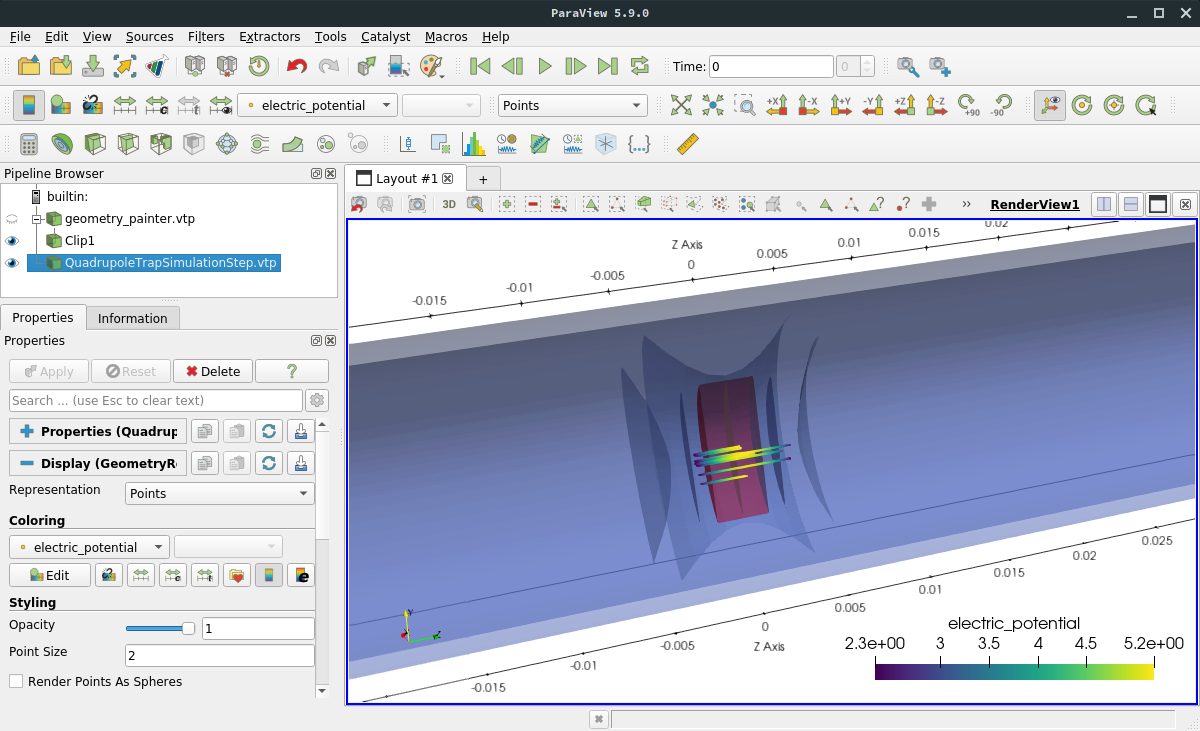
The geometry is shown as colored surfaces according to the configuration in the XML file; the colors are defined by the
<appearance .../> elements. To make the tracks visible, the Slice operation was applied which cuts away one side
of the close surfaces, and the opacity was recuced to 50%. The individual steps are shown as points and colored by
their electric potential.
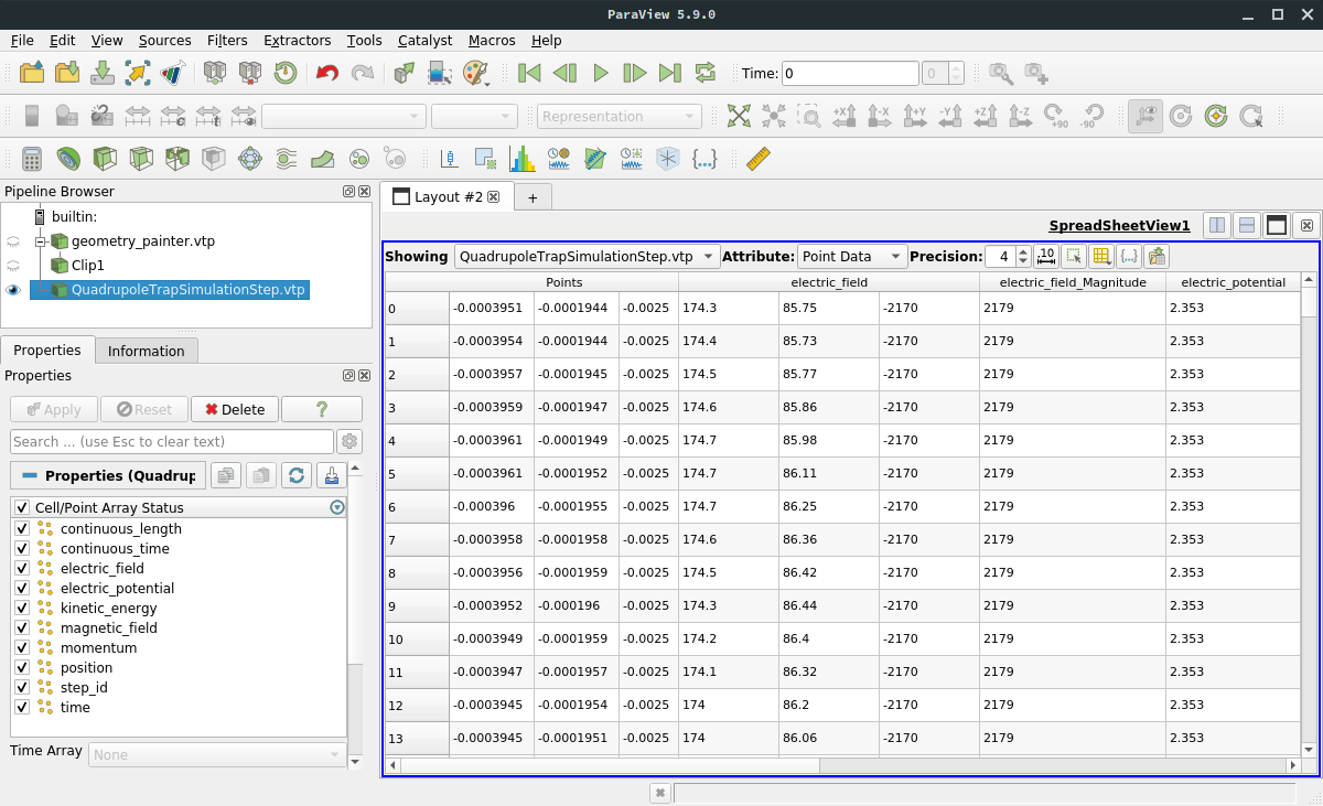
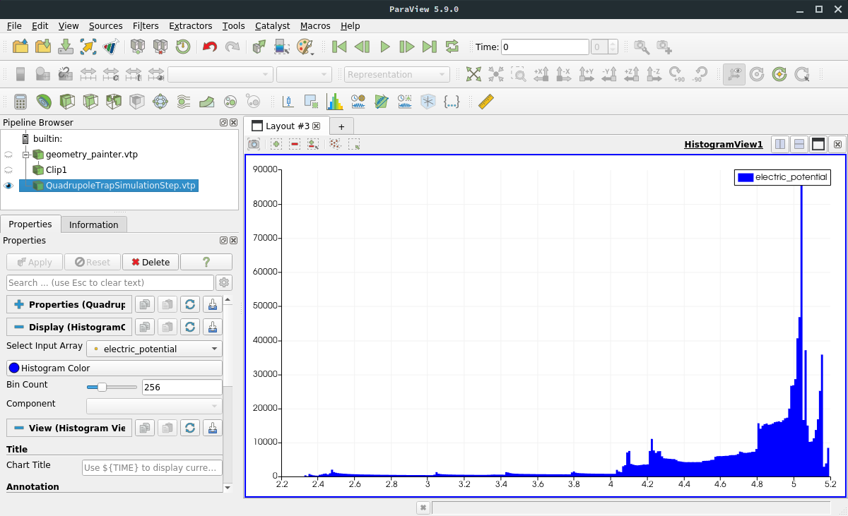
ParaView allows to change the data represenation by choosing different color maps and normalization, applying cuts and other data operations, and combining multiple source files. In addition to 2D and 3D render views, the user can also investigate the underlying data with typical plotting tools like shown here:
For a full documentation, see:
ASCII output files
The ASCII output writer creates a simple, space-separated file that contains all the output values defined in the
configuration file. Each row corresponds to one step and each column to one output field. A new file is created
for each track, with the label Track#.txt added to the configured output file name. This format is useful for
working with plotting tools such as Gnuplot, or for importing or comparing the output to other applications.
A typical output file looks like this:
step_id     continuous_time continuous_length       time    position_x      position_y      position_z
0   3.79467e-13     3.18284e-07     3.79467e-13     -0.000395068    -0.000194398    -0.0025
1   3.79467e-13     3.18288e-07     7.58933e-13     -0.000395383    -0.000194364    -0.0025
2   3.79467e-13     3.18292e-07     1.1384e-12      -0.000395686    -0.000194452    -0.0025
3   3.79467e-13     3.18297e-07     1.51787e-12     -0.000395933    -0.00019465     -0.0025
4   3.79467e-13     3.18301e-07     1.89733e-12     -0.000396085    -0.000194928    -0.0025
5   3.79467e-13     3.18305e-07     2.2768e-12      -0.000396119    -0.000195242    -0.0025
However, because the storage is rather inefficient it should not be used for large-scale simulations. File sizes on the order of several Gigabytes can be easily produced by a typical Monte-Carlo simulation!