Geometry section
Shapes and assemblies
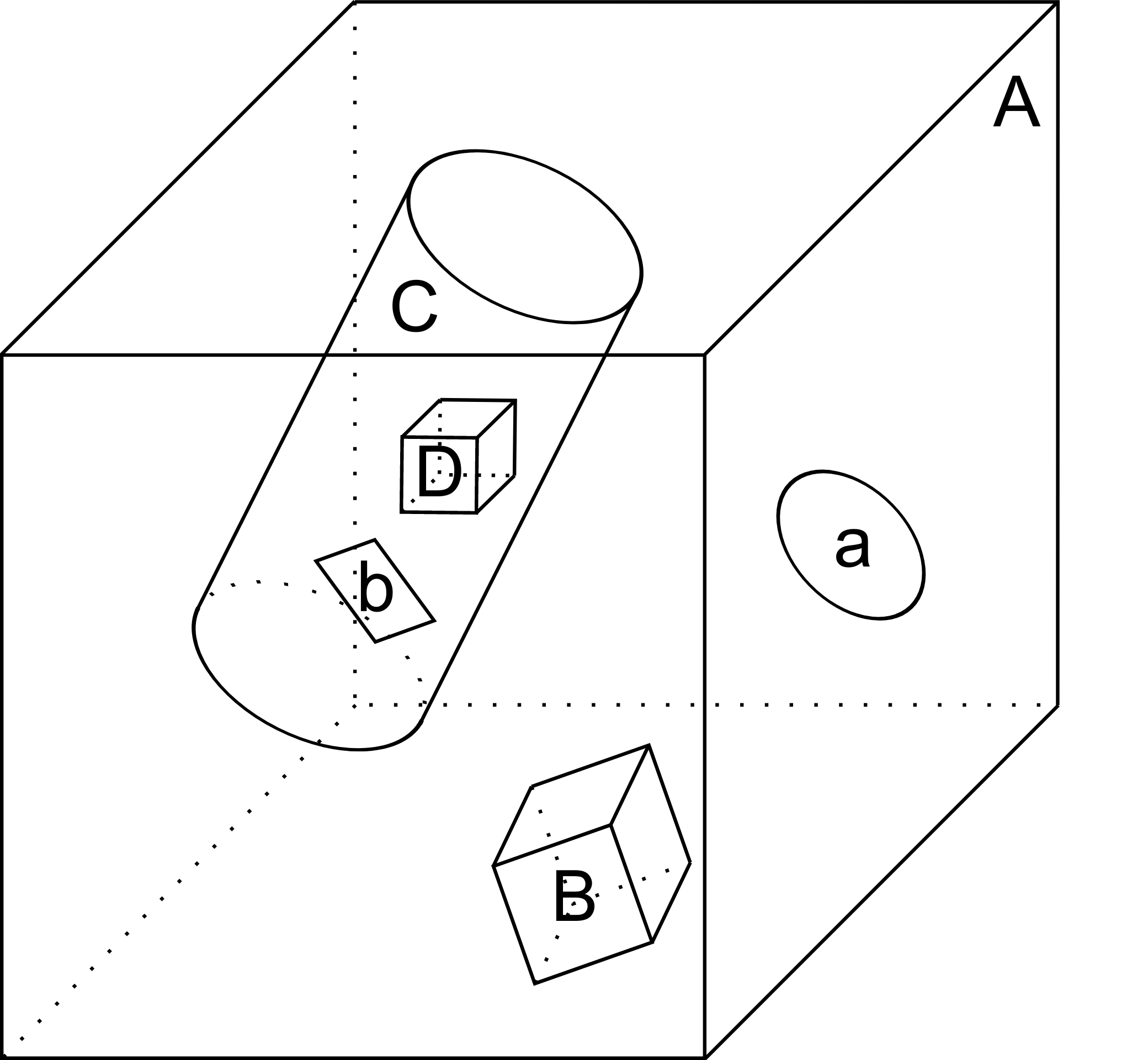
To understand the basics of KGeoBag, let us look at a simple example. A typical simulation geometry may look like the image below, where multiple spaces (B-D) and surfaces (a-b) are assembled and placed in a “world” space A:
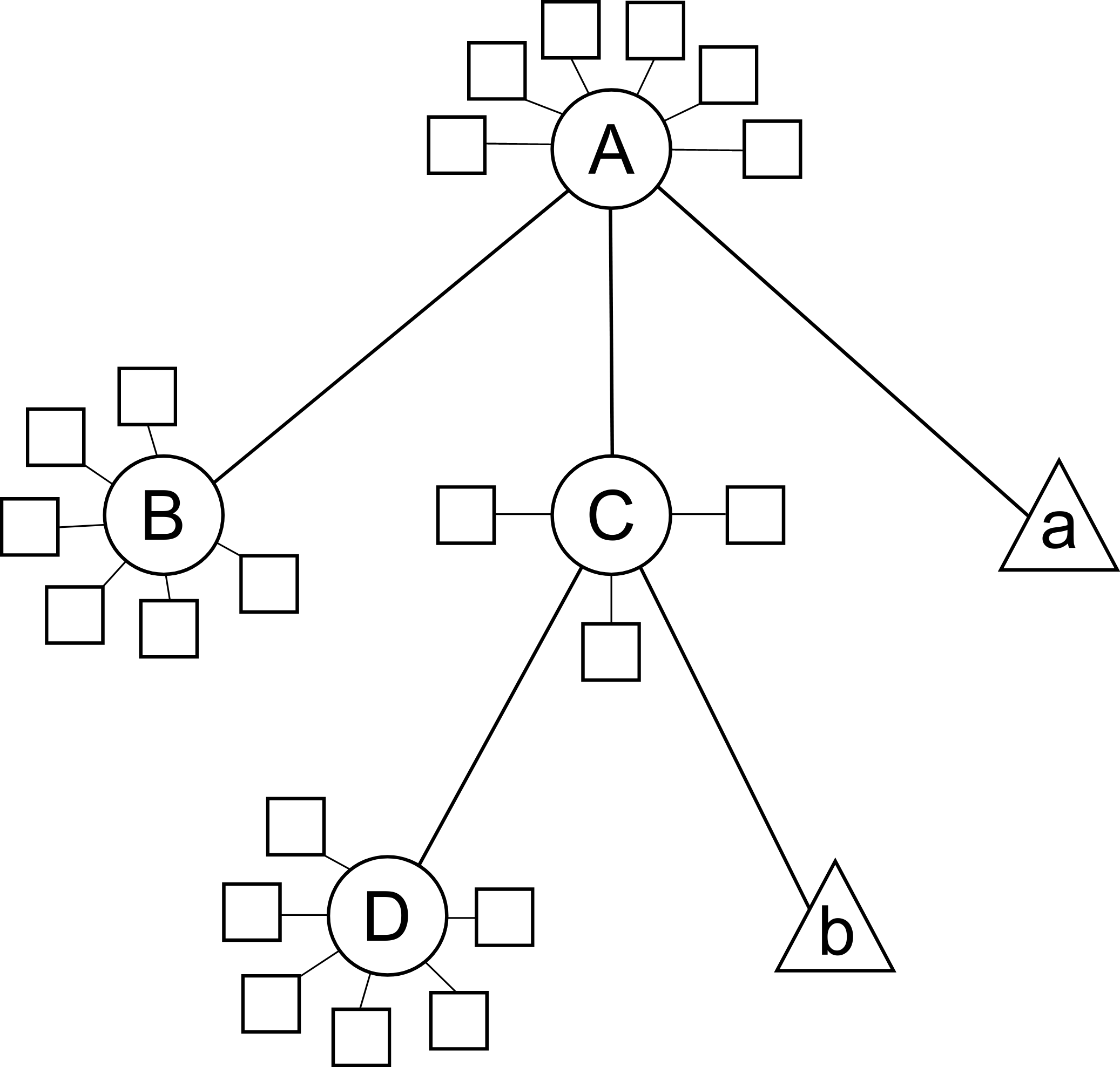
Internally, KGeoBag manages its geometric elements and their relations as a stree structure:
Now, to understand how this works in practice, we’ll look at one of the example files provided with Kassiopeia. Of
the example files provided, the DipoleTrapSimulation.xml has the simplest geometry. It will be explained in detail
below, in order to walk you through a typical geometry configuration.
The geometry section starts off with a description of each shapes involved:
<!-- world -->

<cylinder_space name="world_space" z1="-2." z2="2." r="2."/>

<!-- solenoid -->

<tag name="magnet_tag">
    <cylinder_tube_space
        name="solenoid_space"
        z1="-1.e-2"
        z2="1.e-2"
        r1="0.5e-2"
        r2="1.5e-2"
        radial_mesh_count="30"
    />
</tag>

<!-- ring -->

<tag name="electrode_tag">
    <cylinder_surface
        name="ring_surface"
        z1="-2.0e-2"
        z2="2.0e-2"
        r="2.5e-1"
        longitudinal_mesh_count="200"
        longitudinal_mesh_power="3."
        axial_mesh_count="128"
    />
</tag>

<!-- tube -->

<tag name="electrode_tag">
    <cylinder_surface
        name="tube_surface"
        z1="-1.e-2"
        z2="1.e-2"
        r="0.5e-2"
        longitudinal_mesh_count="200"
        longitudinal_mesh_power="3."
        axial_mesh_count="128"
    />
</tag>

<!-- target -->

<tag name="target_tag">
    <disk_surface name="target_surface" r="1.0e-2" z="0."/>
</tag>

<!-- center -->

<tag name="center_tag">
    <disk_surface name="center_surface" r="2.5e-1" z="0."/>
</tag>
The individual shapes are defined by elements of the common structure:
<some_space name="my_space"/>
<some_surface name="my_surface"/>
where each element is given a name, which it can be referenced with, and additional parameters dependeing on the shape. For example, the disk surface is defined by only two parameters r and z, while other shapes differ.
Tagging system
The tagging system is used to group different elements together, for example by distinguishng between magnet and electrode shapes. These tags will be used later to retrieve elements and pass them to the KEMField module. The general syntax is:
<tag name="my_tag" name="another_tag">
    <shape name="my_shape"/>
</tag>
and tags can be freely combined or re-used.
Assembling elements
The defined shapes are then placed into an assembly of the experiment geometry. Geometric objects are placed by referencing each shape by its given (and unique) name and placing it inside a space. This can be combined with specifying a transformation (relative to the assembly origin) defining the location and orientation of each object. The available transformation types are displacements (defined by a 3-vector), and rotations (defined by an axis-angle pair, or a series of Euler angles using the Z-Y’-Z’’ convention):
<space name="dipole_trap_assembly">
    <surface name="ring" node="ring_surface"/>
    <surface name="center" node="center_surface"/>
    <space name="downstream_solenoid" node="solenoid_space">
        <transformation displacement="0. 0. -0.5"/>
    </space>
    <surface name="downstream_tube" node="tube_surface">
        <transformation displacement="0. 0. -0.5"/>
    </surface>
    <surface name="upstream_target" node="target_surface">
        <transformation displacement="0. 0. -0.48"/>
    </surface>
    <space name="upstream_solenoid" node="solenoid_space">
        <transformation displacement="0. 0. 0.5"/>
    </space>
    <surface name="upstream_tube" node="tube_surface">
        <transformation displacement="0. 0. 0.5"/>
    </surface>
    <surface name="downstream_target" node="target_surface">
        <transformation displacement="0. 0. 0.48"/>
    </surface>
</space>
Here the individual named shapes that were defined earlier are referenced, using the general syntax:
<space name="my_assembly">
    <space name="my_placed_space" node="my_space"/>
</space>
and spaces can be freely nested, which is one of the key features of KGeoBag. Note the difference between the first
space, which does not refer to any shape and just holds the child elements, and the second space which refers to the
shape named my_space through the node attribute. The my_assembly space can be though of as a “virtual space”,
without any reference to a real geometric object.
Finally in the DipoleTrapSimulation.xml file, the full assembly is placed within the world volume:
<space name="world" node="world_space">
    <space name="dipole_trap" tree="dipole_trap_assembly"/>
</space>
The world volume is a crucial part of any geometry, since it defines the outermost “root” space in which all other
elements must be placed. Note that in this case, the space named dipole_trap_assembly is referenced through the
tree attribute (and not node, as you might expect.) This is due to the fact that the assembly is a “virtual” space
that just holds its child elements, but does not refer to an actual object. Make sure to keep this in mind for your
own geometry configurations!
Transformations
It should be noted that transformations applied to an assembly are collectively applied to all of the geometric elements within the assembly. For example, placing the dipole trap assembly within the world volume as:
<space name="world" node="world_space">
    <space name="dipole_trap" tree="dipole_trap_assembly">
        <transformation rotation_euler="90. 0. 0." displacement="0 0 1.0"/>
    </space>
</space>
would rotate the whole assembly by 90 degrees about the z-axis, and then displace it by 1 meter along the z-axis.
Assemblies may be nested within each other, and the coordinate transformations which are associated with the placement of each assembly will be appropriately applied to all of the elements they contain. This makes it very intuitive to create complex geometries with multiple displacements and rotations, because it resembles the behavior of real-world objects (i.e. turning an assemble object by some amount will also turn all parts inside by the same amount, relative to the outside coordinate system.)
Especially for rotations, it should be noted that it makes a difference if they are applied in the assembly before or after placing child elements. Consider the following example:
<disk_surface name="disk_surface" r="1.0" z="0."/>

<space name="world">
    <space name="assembly_1">
        <surface name="placed_disk" node="disk_surface"/>
        <transformation rotation_euler="0. 30. 0." displacement="0 0 -1.0"/>
    </space>
    <space name="assembly_2">
        <transformation rotation_euler="0. 30. 0." displacement="0 0 1.0"/>
        <surface name="placed_disk" node="disk_surface"/>
    </space>
</space>
In this case, the placed_disk in in the first assembly will be tilted relative to the world volume, while the
disk in the second assembly will not! This can be verified easily with one of the geometry viewers, which are explained
in section KGeoBag Visualization. The reason for this behavior is that in the second case, the rotation was
applied before placing the surface inside the assembly, and so it is not propagated to the shape. This is on purpose,
because it allows to transform the origin and orientation of the reference system before assembling elements.
It is best to think of the <transformation> elements as commands that are executed during XML initialization, while
the geometry is assembled. It should be clear then that the two example assemblies yield different results.
Extensions
In order to give physical properties to the geometry elements that have been constructed and placed, they must be associated with extensions. The currently available extensions are meshing (axially or rotationally symmetric, or non-symmetric), visualization properties, electrostatic boundary conditions (Dirichlet or Neumann surfaces), and magnetostatic properties of solenoids and coils (current density and number of windings.)
A simple extension example is specifying the color and opacity of a shape for its display in a VTK visualization window as follows:
<appearance name="app_magnet" color="0 255 127 127" arc="72" surfaces="world/dipole_trap/@magnet_tag"/>
This example tells the visualization that any shape given the tag magnet_tag should be colored with an RGBA color
value of (0,255,127,127), where all values are given in the range 0..255 and the fourth value defines the shape’s
opacity. If you have VTK enabled you may wish to experiment with the changes introduced by modifying these parameters.
When using the ROOT visualization, the appearance settings will be ignored.
In the line above, you also find an example of referencing tags throught the @tag_name syntax. Generally the
placed shapes can be referenced through a XPath-like syntax that defines the location in the geometry tree, starting
at the “root” volume (which is typically called world.) This usually works with all spaces and surfaces
attributes of the XML elements.
The tagging feature is very useful for applying properties to many different elements at once. To do this, each element
which is to receive the same extension must share the same tag. There is no limit to the number of tags an geometric
element may be given. For example, given the dipole trap geometry as specified, one may associate an axially symmetric
mesh with all elements that share the tag electrode_tag with the line:
<axial_mesh name="mesh_electrode" surfaces="world/dipole_trap/@electrode_tag"/>
This specifies that any geometric shape with the tag electrode_tag that is found within the world/dipole_trap
space should be giving an axial mesh extension (i.e. it will be divided into a collection of axially symmetric objects
like cones, cylinders, etc.) This axial mesh will be later used by the field solving routines in KEMField. However, a
tag is not strictly necessary to apply an extension. For example, if we wished to generate an axial mesh for everything
within the world volume we would write:
<axial_mesh name="mesh_electrode" surfaces="world/#"/>
or, if we wished to single out the ring_surface shape by specifying its full path we would write:
<axial_mesh name="mesh_electrode" surfaces="world/dipole_trap/ring"/>
Meshing is critical for any problem with involves electrostatic fields. The type of mesh depends on the symmetry of the
geometry. For completely axially-symmetric geometries, the axial_mesh is recommended so that the zonal harmonics
field computation method may be used. For completely non-symmetric (3D) geometries, the mesh type would be specified as
follows:
<mesh name="mesh_electrode" surfaces="world/dipole_trap/@electrode_tag"/>
Because of the very shape-specific nature of the deterministic meshing which is provided by KGeoBag, parameters
(mesh_count and mesh_power) describing how the mesh is to be constructed are given when specifying the shapes
themselves. That being said, the mesh associated with a specific shape will not be constructed unless the extension
statement is present.
It is possible to define multiple meshes side by side, e.g. if the simulation can be configured axially-symmetric or non-symmetric. In this case, both meshes will be available for KEMField calculations regardless of the symmetry setting. Note that the axial mesh cannot handle any non-symmetric elements, and these will be simply ignored.
Another important extension for field calculations is the specification of boundary conditions. For example, when solving the Laplace boundary value problem via KEMField, one may specify that a particular surface exhibit Dirichlet boundary conditions where a particular voltage is applied to the surface through the use of the following extension:
<electrostatic_dirichlet name="electrode_ring" surfaces="world/dipole_trap/ring" value="-10."/>
Where value="-10" signifies that this surface has a potential of -10 volts. This is the standard case for defining
(metallic) electrode surfaces in a simulation, and a typical scenario for the boundary-element method (BEM). It is also
possible to define Neumann boundary conditions, which are typically used for insulating materials.
Similar to the electrode setup, one can define a magnet system that provides a magnetostatic field for the simulation. For example, one may specify a solenoid electromagnet with the appropriate parameters:
<electromagnet name="electromagnet_upstream_solenoid" spaces="world/dipole_trap/upstream_solenoid" current="{22.3047 * 20000}"/>
which references a space named upstream_solenoid with a total current of 22.3047 amps times 20000 turns. The
electric current and the number of turns can also be specified separately for added clarity:
<electromagnet name="electromagnet_upstream_solenoid" spaces="world/dipole_trap/upstream_solenoid" current="22.3047" num_turns="20000"/>
The cylinder tube space is one of the supported shapes for electromagnets and describes a solenoid geometry. Other supported shapes are the cylinder surface, describing a simple coil, and the rod space, describing a single wire.
For further demonstrations of the possible geometry extensions please see the provided example XML files located at GitHub: KGeoBag/Source/XML/Examples.